Automatic Video Annotation – Software Description

Project By: Krishna Adatrao
Evaluation: Tata Consultancy Services

Deep learning is an artificial intelligence function that imitates the workings of the  human brain in processing data and creating patterns for use in decision making. Deep learning is a subset of machine learning in artificial intelligence (AI) that has networks capable of learning unsupervised from data that is unstructured or unlabeled.

Deep learning architectures such as deep neural networks, deep belief networks, recurrent neural networks and Convolutional neural networks have been applied to fields including computer vision, speech recognition, natural language processing, audio recognition, social network filtering, machine translation, bio-informatics, drug design, medical image analysis, material inspection and board game programs, where they have produced results comparable to and in some cases surpassing human expert performance.

Deep learning is a key technology behind driver-less cars, enabling them to recognize a stop sign, or to distinguish a pedestrian from a lamppost. It is the key to voice control in consumer devices like phones, tablets, TVs, and hands-free speakers.

In deep learning, a computer model learns to perform classification tasks directly from images, text, or sound. Deep learning models can achieve state-of-the-art accuracy, sometimes exceeding human-level performance. Models are trained by using a large set of labeled data and neural network architectures that contain many layers.

While deep learning was first theorized in the 1980s, there are two main reasons it has only recently become useful:

1. Deep learning requires large amounts of labeled data. For example, driver-less car development requires millions of images and thousands of hours of video.
2. Deep learning requires substantial computing power. High-performance GPU’s have a parallel architecture that is efficient for deep learning. When combined with clusters or

cloud computing, this enables development teams to reduce training time for a deep learning network from weeks to hours or less.

A neural network consists of several different layers  such  as  the input layer,  at  least  one hidden layer,  and  an output layer.  They  are  best  used  in  object  detection   for recognizing patterns such as edges(vertical/horizontal), shapes, colours, and textures.The hidden layers are Convolutional layers in this type of neural network which acts like a filter that first receives input, transforms it using a specific pattern/feature, and sends it to the next layer. With more Convolutional layers, each time a new input is sent to the next Convolutional layer, they are changed in different ways. For example, in the first Convolutional layer, the filter may identify shape/colour in a region (i.e. brown), and the next one may be able to conclude the object it really is (i.e. an ear or paw), and the last Convolutional layer may classify the object as a dog. Basically, as more and more layers the input goes through, the more sophisticated patterns the future ones can detect. CNNs eliminate the need for manual feature extraction, so you do not need to identify features used to classify images. The CNN works by extracting features directly from images. The relevant features are not pretrained, they are learned while the network trains on a collection of images. This automated feature extraction makes deep learning models highly accurate for computer vision tasks such as object classification.

In the case of a fixed rigid object in an image, only one example may be needed, but more generally multiple training examples are necessary to capture certain aspects of class variability

Convolutional implementation of the sliding windows Before we discuss the implementation of the sliding window using convents, let us analyze how we can convert the fully connected layers of the network into Convolutional layers. Fig.4.1 shows a simple Convolutional network with two fully connected layers each of shape.

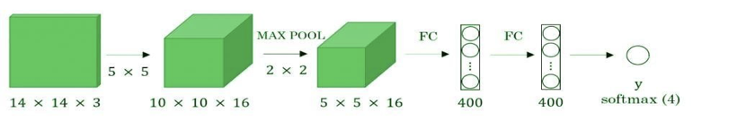
Figure 4.1 simple convolution network

A fully connected layer can be converted to a Convolutional layer with the help of a 1D Convolutional layer. The width and height of this layer is equal to one and the number of filters are equal to the shape of the fully connected layer. An example of this is shown in Fig 4.2.

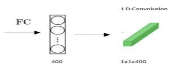
Figure 4.2

 We can apply the concept of conversion of a fully connected layer into a Convolutional layer to the model by replacing the fully connected layer with a 1-D Convolutional layer. The number of filters of the 1D Convolutional layer is equal to the shape of the fully connected layer. This representation is shown in Fig 4.3. Also, the output softmax layer is also a Convolutional layer of shape (1, 1, 4), where 4 is the number of classes to predict.

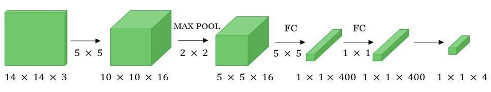
Figure 4.3

Now, let’s extend the above approach to implement a Convolutional version of the sliding window. First, letus consider the ConvNet that we have trained to be in the following representation (no fully connected layers).

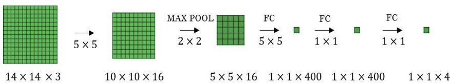
Figure 4.4

Let’s assume the size of the input image to be 16 × 16 × 3. If we are using the sliding window approach, then we would have passed this image to the above ConvNet four times, where each time the sliding window crops the part of the input image matrix of size 14 × 14 × 3 and pass it through the ConvNet. But instead of this, we feed the full image (with shape 16 × 16

× 3) directly into the trained ConvNet in below figure. This result will give an output matrix of shape 2 × 2 × 4. Each cell in the output matrix represents the result of the possible crop and the classified value of the cropped image. For example, the left cell of the output matrix(the green one) in Fig. 4.5 represents the result of the first sliding window. The other cells in the matrix represent the results of the remaining sliding window operations.

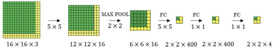
Figure4.5

The stride of the sliding window is decided by the number of filters used in the Max Pool layer. In the example above, the Max Pool layer has two filters, and for the result, the sliding window moves with a stride of two resulting in four possible outputs to the given input. The main advantage of using this technique is that the sliding window runs and computes all values simultaneously. Consequently, this technique is really fast. The weakness of this technique is that the position of the bounding boxes is not very accurate.

YOLO is a new and a novel approach to object detection. Prior work on object detection repurposes classifiers to perform detection. YOLO frames object detection as a regression problem to spatially separated bounding boxes and associated class probabilities. A single neural network predicts bounding boxes and class probabilities directly from full images in one evaluation. Since the whole detection pipeline is a single network, it can be optimized end-to-end directly on detection performance.

Unlike sliding window and region proposal-based techniques, YOLO sees the entire image during training and test time so it implicitly encodes contextual information about classes as well as their appearance. Fast R – CNN, a top detection method, mistakes background patches in an image for objects because it cannot see the larger context. YOLO makes less than half the number of background errors compared to Fast R – CNN.

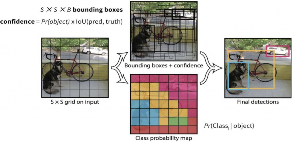
Figure 4.6 You Only Look Once (YOLO)

Jupyter Notebook

The Jupyter Notebook is an open source web application that you can use to create and share documents that contain live code, equations, visualizations, and text. Jupyter Notebook is maintained by the people at Project Jupyter. Jupyter Notebooks are a spin-off project from the IPython project, which used to have an IPython Notebook project itself. The name, Jupyter, comes from the core supported programming languages that it supports: Julia, Python, and R. Jupyter ships with the IPython kernel, which allows you to write your programs in Python, but there are currently over 100 other kernels that you can also use.

TensorFlow

TensorFlow is a free and open-source software library for data flow and differentiable programming across a range of tasks. It is a symbolic math library, and is also used for machine learning applications such as neural networks. It is used for both research and production at Google. TensorFlow was developed by the Google Brain team for internal Google use. It was released under the Apache License 2.0 on November 9, 2015.

KERAS

Kerasis an open-source neural-network library written in Python. It is capable of running on top of TensorFlow, Microsoft Cognitive Toolkit, Theano, or PlaidML. Designed to enable fast experimentation with deep neural networks, it focuses on being user-friendly, modular, and extensible. It was developed as part of the research effort of project ONEIROS (Open-ended Neuro Electronic Intelligent Robot Operating System), and its primary author and maintainer is François Chollet, a Google engineer. Chollet also is the author of the XCeption deep neural network model. In 2017, Google’s TensorFlow team decided to support Kerasin TensorFlow’s corelibrary.

OpenCV

OpenCV (Open Source Computer Vision Library) is an open source computer vision and machine learning software library. OpenCV was built to provide a common infrastructure for computer vision applications and to accelerate the use of machine perception in the commercial products. Being a BSD-licensed product, OpenCV makes it easy for businesses to utilize and modify the code. The library has more than 2500 optimized algorithms, which includes a comprehensive set of both classic and state-of-the-art computer vision and machine learning algorithms. These algorithms can be used to detect and recognize faces, identify objects, classify human actions in videos, track camera movements, track moving objects, extract 3D models of objects, produce 3D point clouds from stereo cameras, stitch images together to produce a high resolution image of an entire scene, find similar images from an image database, remove red  eyes from images taken using flash, follow eye movements, recognize scenery and establish markers to overlay it with augmented reality, etc. OpenCV has more than 47 thousand people of user community and estimated number of downloads exceeding 18 million. The library is used extensively in companies, research groups and by governmental bodies.

PILLOW

Pillow, previously known as PIL(Python Imaging Library) is used for image manipulations. It adds image processing capabilities to your Python interpreter. This library provides extensive file format support, an efficient internal representation, and fairly powerful image processing capabilities. The core image library is designed for fast access to data stored in a few basic pixel formats. It should provide a solid foundation for a general image processing tool.

NUMPY

NumPy, which stands for Numerical Python, is a library consisting of multidimensional array objects and a collection of routines for processing those arrays. Using NumPy, mathematical and logical operations on arrays can be performed.

Matplotlib

Matplotlib is an amazing visualization library in Python for 2D plots of arrays. Matplotlib is a multi-platform data visualization library built on NumPy arrays and designed to work with the broader  SciPy stack.  It  was  introduced  by  John  Hunter  in  the  year  2002.  Matplotlib is a plottinglibraryfor the Python programming language and its numerical  mathematics  extension NumPy. It provides an object-oriented API for embedding plots into applications using general-purpose GUI toolkits like Tkinter, wxPython, Qt, orGTK+.

SciPy

SciPy is a library that uses NumPy for more  mathematical  functions. SciPy  uses NumPy arrays  as  the  basic  data  structure,  and  comes  with  modules  for  various   commonly used tasks in scientific programming, including linear algebra, integration (calculus), ordinary differential equation solving, and signal processing.

Pandas

pandas is a Python package providing fast, flexible, and expressive data structures designed to make working with “relational” or “labeled” data both easy and intuitive. It aims to be the fundamental high-level building block for doing practical, real world data analysis in Python.

Struct

This module performs conversions between Python values and C structs represented as Python bytes objects. This can be used in handling binary data stored in files or from network connections, among other sources. It uses Format Strings as compact descriptions of the layout of the C structs and the intended conversion to/from Python values.

Data set

A data set is a collection of related, discrete items of related data that may be accessed individually or in combination or managed as a whole entity.

A data set is organized into some type of data structure. In a database, for example, a data set might contain a collection of business data (names, salaries, contact information, sales figures, and so forth). The database itself can be considered a data set, as can bodies of data within it related to a particular type of information, such as sales data for a particular corporate department.

Pascal Visual Object Classes(VOC)

One of the most important tasks in computer vision is to label the data. There are several tools available where you can load the images, label the objects using per-instance segmentation. This aids in precise object localization using bounding boxes or masking using polygons. This information is stored in annotation files.

Figure 4.7  Sample Pascal VOC

Pascal VOC provides standardized image data sets for object detection which contains 20 classes.

Difference between COCO and Pascal VOC data formats will quickly help understand the two data formats

1. Pascal VOC is an XML file, unlike COCO which has a JSON file.

1. In Pascal VOC we create a file for each of the image in the dataset. In COCO we have one file each, for entire dataset for training, testing and validation.

1. The bounding Box in Pascal VOC and COCO data formats are different

COCO Bounding box: (x-top left, y-top left, width, height)

Pascal VOC Bounding box: (x min – top left, y min – top left, x max – bottom right, y max -bottom right) List of Classes in Pascal VOC:

1. Background
2. Aeroplane
3. Bicycle
4. Bird
5. Boat
6. Bottle
7. Bus
8. Car
9. Cat
10. Chair
11. Cow
12. Diningtable
13. Dog
14. Horse
15. Motorbike
16. Person
17. Potted plant Sheep Sofa Train T.V. Monitor

Some of the key tags for Pascal VOC are explained below

Folder:

Folder that contains the images

Filename:

Name of the physical file that exists in the folder

Size:

It contain the size of the image in terms of width, height and depth. If the image is black and white then the depth will be 1. For color images, depth will be3

Object:

It contains the object details. If you have multiple annotations then the object tag with its contents is repeated. The components of the object tags are

1. Name
2. Pose
3. Truncated
4. Difficult
5. Bounding Box

Training, labels, and inference

• During training, an image classification model is fed images and their associated labels. Each label is the name of a distinct concept, or class, that the model will learn to recognize.
• Given sufficient training data (often hundreds or thousands of images per label), an image classification model can learn to predict whether new images belong to any of the classes it has been trained on. This process of prediction is calledinference.
• To perform inference, an image is passed as input to a model. The model will then output an array of probabilities between 0 and1.

Implemented this model as a Convolutional neural network and evaluate it on the PASCAL VOC detection dataset. The initial Convolutional layers of the network extract feature from the image while the fully connected layers predict the output probabilities and coordinates. Our network architecture is inspired by the Google Net model for image classification. Our network has 24 Convolutional layers followed by 2 fully connected layers. Instead of the inception modules used by Google Net, we simply use 1_1 reduction layer followed by 3_3 Convolutional layers. We also train a  fast version of YOLO designed to push the boundaries of fast object detection. Fast YOLO uses a neural network with fewer Convolutional layers (9 instead of 24) and fewer filters in those layers. Other than the size of the network, all training and testing parameters are the same between YOLO and Fast YOLO. The final output of our network is the 7 *7* 30 tensor of predictions as shown in the architecture below.

CNN Architecture

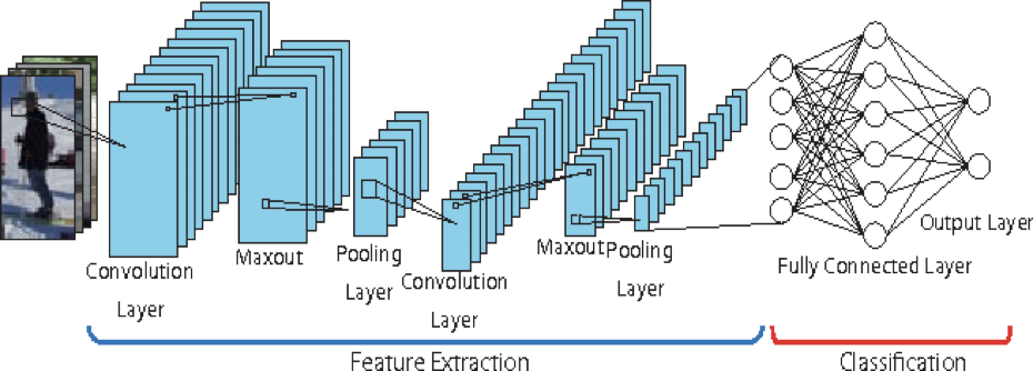
Figure 5.1 Conventional CNN architecture

YOLO Model Architecture

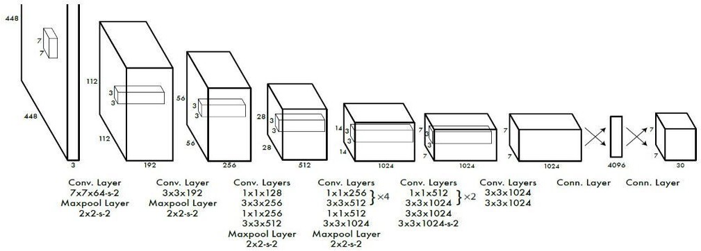
Figure 5.2 The YOLO Architecture.

Our detection network has 24 Convolutional layers followed by 2 fully connected layers. Alternating 1 * 1 Convolutional layers reduce the features space from preceding layers. We retrain the Convolutional layers on the Image Net classification task at half the resolution (224 _ 224 input image) and then double the resolution for detection.

The above model consists of 24 Convolutional layers followed by 2 fully connected layers.Alternating1×1Convolutional layers reduce the features space from preceding layers. (1×1) conv has been used used in Google Net for reducing number of parameters.). Fast YOLO fewer Convolutional layers (9 instead of 24) and fewer filters in those layers.